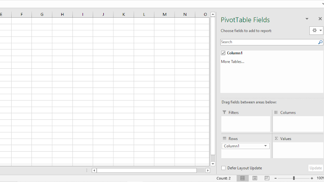
Hello everyone, How are you all doing? This brief tutorial will show us how to create a Pivot Chart in Microsoft excel. Pivot chart helps users to present and visualize the raw data in a better way. Creating a Pivot chart in Excel is quite a straightforward process so follow this article till the end.
Read more: How to make PDF in mobile
How to Create a Pivot Chart in Excel
To create a pivot chart in Excel, follow the steps given below:
Step-1: Open Microsoft excel and select the blank sheet.
Step-2: Enter raw data in the blank sheet.
Step-3: Now, select the cell in a range or table.
Step-4: Go to the insert tab and click on the pivot chart.
Step-5: Choose where you want the PivotChart to be placed. After selecting, click on Ok.
Step-6: Now, select the field to display in the PivotChart.
In this way, you can successfully create a PivotChart in Microsoft excel.
Thank you guys for reading out this article till the end. I do hope that this article will really help you in creating a pivot chart in Excel. If you feel any sort of problem with the above steps, you can contact us by commenting n this article.
Read more:


Post a Comment